Plot Coverage Map with Candidate Gene Annotations

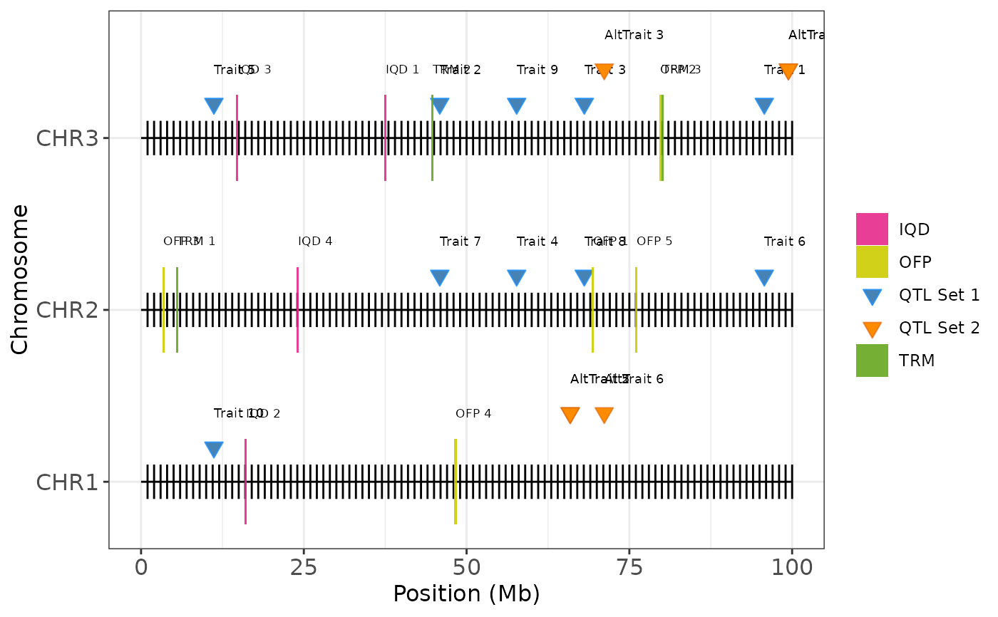
Visualizes chromosome positions, QTLs, and gene of interest annotations on a multi-chromosome physical map. Useful for displaying genomic regions of interest, highlighting genetic features such as QTLs and candidate genes or protein families.

Usage

plot_coverage_annotate(
  map,
  limits = NULL,
  qtls = NULL,
  qtls2 = NULL,
  prot1 = NULL,
  prot2 = NULL,
  prot3 = NULL,
  labels = NULL,
  protein_colors = NULL,
  qtl_labels = c("QTLs Full Panel", "QTLs Table Beet Only"),
  qtl_colors = c("#1E90FF", "#D95F02"),
  show_labels = TRUE
)

Arguments

map

A data frame with at least two columns: chrom (chromosome ID) and position (genomic coordinate in base pairs). This forms the base map.

limits

Optional data frame with chromosome end positions. If NULL, limits are computed automatically.

qtls

Optional data frame of QTLs. Should contain chrom, position, and optionally trait.

qtls2

Optional second QTL set (e.g., from another population). Same format as qtls.

prot1

First protein/gene annotation data frame. Should contain chrom, position, and name.

prot2

Second protein/gene annotation data frame. Same format as prot1.

prot3

Third protein/gene annotation data frame. Same format as prot1.

labels

Optional vector of labels (length 1–3) for protein layers (e.g., c("OFP", "IQD", "TRM")).

protein_colors

Optional vector of fill colors for proteins, matching the order in labels.

qtl_labels

Character vector of length 2 defining the legend labels for qtls and qtls2.

qtl_colors

Character vector of length 2 defining the fill colors used for the two QTL types.

show_labels

Logical; whether to display text labels for QTL traits and protein names (default: TRUE).

Value

A ggplot object showing the annotated chromosome map.

Examples

# Simulated example
set.seed(123)

# Create basic map for 3 chromosomes
example_map <- data.frame(
  chrom = rep(paste0("CHR", 1:3), each = 100),
  position = rep(seq(1e6, 100e6, length.out = 100), 3)
)

# QTL sets
example_qtls <- data.frame(
  chrom = sample(paste0("CHR", 1:3), 10, replace = TRUE),
  position = runif(5, min = 1e6, max = 100e6),
  trait = paste("Trait", 1:10)
)
example_qtls2 <- data.frame(
  chrom = sample(paste0("CHR", 1:3), 6, replace = TRUE),
  position = runif(3, min = 1e6, max = 100e6),
  trait = paste("AltTrait", 1:6)
)

# Protein annotations
ofp_data <- data.frame(
  chrom = sample(paste0("CHR", 1:3), 5, replace = TRUE),
  position = runif(5, 1e6, 100e6),
  name = paste("OFP", 1:5)
)

iqd_data <- data.frame(
  chrom = sample(paste0("CHR", 1:3), 4, replace = TRUE),
  position = runif(4, 1e6, 100e6),
  name = paste("IQD", 1:4)
)

trm_data <- data.frame(
  chrom = sample(paste0("CHR", 1:3), 3, replace = TRUE),
  position = runif(3, 1e6, 100e6),
  name = paste("TRM", 1:3)
)

# Plot annotated coverage map
plot_coverage_annotate(
  map = example_map,
  qtls = example_qtls,
  qtls2 = example_qtls2,
  prot1 = ofp_data,
  prot2 = iqd_data,
  prot3 = trm_data,
  labels = c("OFP", "IQD", "TRM"),
  qtl_labels = c("QTL Set 1", "QTL Set 2"),
  qtl_colors = c("steelblue", "darkorange"),
  show_labels = TRUE
)