Introduction
This article demonstrates how to process, clean, and recode (phase)
SNP markers from a VCF file to generate genotype matrices compatible
with genetic mapping workflows. We will use helper functions from the
geneticMapR package as well as dependencies such as
MapRtools, VariantAnnotation, and
Rsamtools. The example focuses on an F2 population, where
genotype recoding is based on founder descent.
Setup
We will need a series of packages, below we show how to install them if needed. (geneticMapR needs to be installed)
# Ensure devtools is available for GitHub installs
load_or_install_cran("devtools")

# Install/load GitHub packages
load_or_install_github("MapRtools", "jendelman/MapRtools")

# Install/load CRAN packages
load_or_install_cran("ggplot2")
load_or_install_cran("tidyr")
load_or_install_cran("tidyverse")
load_or_install_cran("parallel")
load_or_install_cran("BiocManager")


# Variant Annotation Package
BiocManager::install("VariantAnnotation")
load_or_install_cran("VariantAnnotation")
Load and Explore VCF File
The VCF file is somewhat large (19.8 MB) to be included as a system
file. geneticMapRFiles
is a data-only repository that will help us save data and run through
examples without much issues. Let’s get a local copy of the VCF file
using utils::download.file()
# Let's define our URL from the data repository that accompanies this R package
vcf_url <- "https://raw.githubusercontent.com/vegaalfaro/geneticMapRFiles/main/vcf/SNP_updated_IDs_sorted2.vcf.gz"

# Download file
if (!file.exists("local_copy.vcf.gz")) {
  download.file(vcf_url, destfile = "local_copy.vcf.gz")
}
The code below loads the vcf file using the function readVcf.
# Let's read the vcf into our environment
vcf2 <- VariantAnnotation::readVcf("local_copy.vcf.gz", genome = "unknown")
Let’s explore the vcf file. The VCF contains several fields including GT (genotype), DP (depth), GQ (genotype quality) and PL (sample-level annotations)
Extract Genotype and Coverage Information
Let’s extract the genotype and depth which are saved in the GT and DP fields using VariantAnnotation’s geno function.
Once extracted, we can estimate depth statistics.
summary(as.numeric(DP))
#>    Min. 1st Qu.  Median    Mean 3rd Qu.    Max.
#>    0.00   19.00   27.00   30.84   39.00 1656.00
Convert Genotype Call to Dosage
If we inspect the GT object,
GT[1:3, 1:3]
#>             7001-F1-Beta-H9 2001-F2-Beta-A10 2002-F2-Beta-B10
#> CHR7_192222 "1/0"           "0/1"            "1/1"
#> CHR7_192239 "0/0"           "0/0"            "0/0"
#> CHR7_192241 "0/0"           "0/0"            "0/0"
genotypes are coded as "0/0", "0/1", or
"1/1", representing the maximum likelihood call:
0 for the reference (REF) allele and 1 for the
alternate (ALT) allele. For example:
-
"0/0"is a dosage of 0 ALT alleles, -
"0/1"or"1/0"is a dosage of 1 ALT allele and -
"1/1"corresponds to a dosage of 2 ALT alleles.
The convert_to_dosage family
of functions in geneticMapR handles this conversion
easily. For polyploids (e.g., "0/0/0/0"), check out
convert_to_dosage_advanced and
convert_to_dosage_flex.
Let’s convert the genotype calls into dosages:
geno_1629 <- convert_to_dosage_flex(GT)Let’s take a look at the conversion.
geno_1629[1:3, 1:3]
#>             7001-F1-Beta-H9 2001-F2-Beta-A10 2002-F2-Beta-B10
#> CHR7_192222               1                1                2
#> CHR7_192239               0                0                0
#> CHR7_192241               0                0                0
We have converted to dosage from allele format call.
Filter Markers and Individuals by Missing Data
The function filter_missing_geno() takes a genotype
matrix with rows representing genetic markers and columns representing
individuals. The geno_matrix argument specifies the
genotype matrix.
The threshold argument allows to specify the max
proportion of missing data before an individual or marker is removed.
Ranges from 0 to 1 and the default is 0.10.
Let’s filter by markers first and accept 10% missing
data.
result <- filter_missing_geno(geno_matrix = geno_1629,
                              threshold = 0.10,
                              filter_by = "markers")
#> 0 markers removed (Threshold: 0.1)

# Extract our result
filtered_geno <- result$filtered_geno
We can see that no marker was removed. Our markers have all less than 10% missing data. We can confirm it using a plot.
# Prepare data
missing_values <- base::as.data.frame(result$pct_missing)
colnames(missing_values) <- "missing"

# Visualize missingness
ggplot(missing_values, aes(x = missing)) +
  geom_histogram()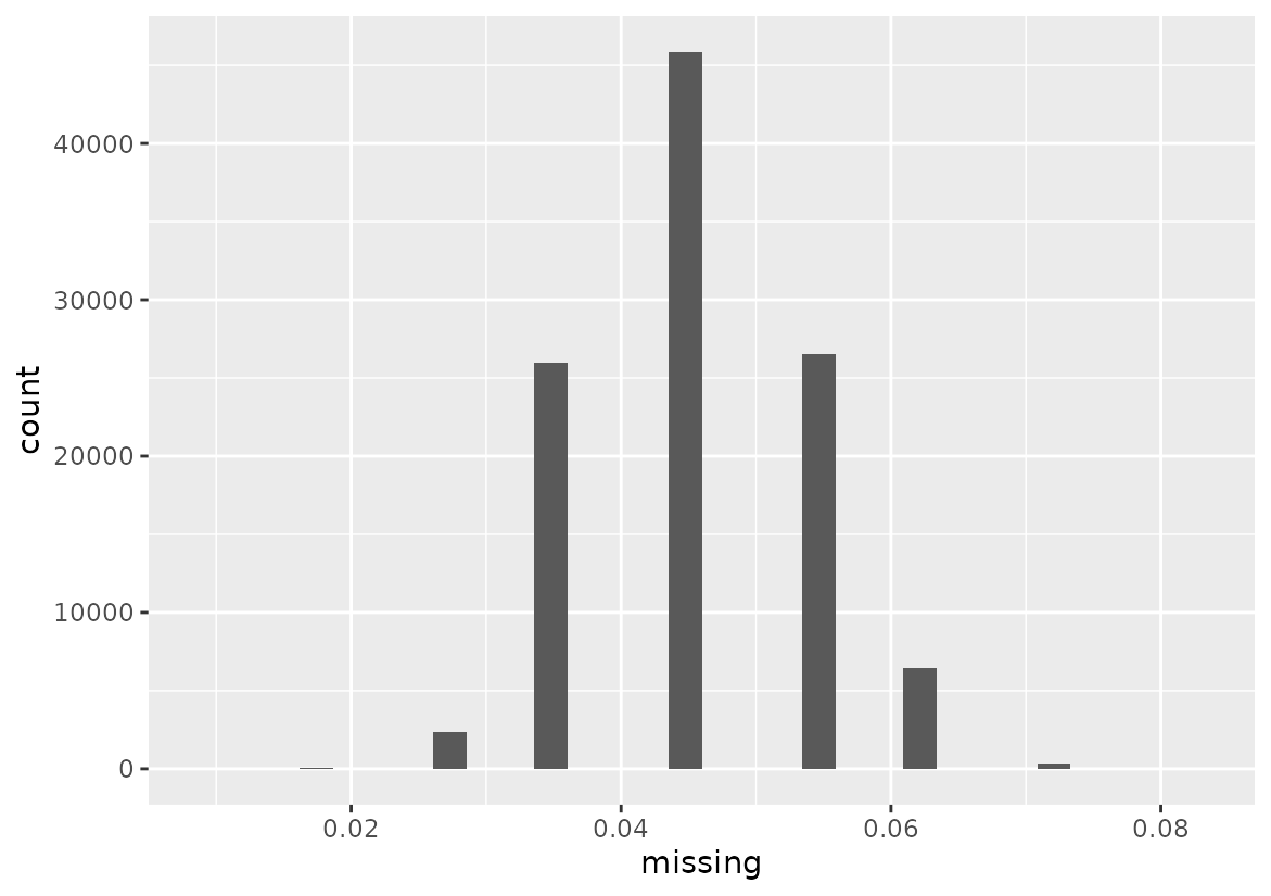
We can also filter by missing data per individuals.
geno_missing_filtered <- filter_missing_geno(filtered_geno,
                                             threshold = 0.10,
                                             filter_by = "individuals")
#> 7 individuals removed (Threshold: 0.1)
filtered_geno <- geno_missing_filtered$filtered_geno
The function created a message letting us know that 7 individuals were removed as they have data that exceeds the 0.1 threshold.
Let’s see an example on how to access the results.
# Access outputs
filtered_geno <- geno_missing_filtered$filtered_geno # Filtered geno matrix
missing_values <- base::as.data.frame(geno_missing_filtered$pct_missing) #
colnames(missing_values) <- "missing"

# Removed individuals
removed_individuals <- data.frame(ind = geno_missing_filtered$removed_individuals)
Let’s see which individuals were removed
print(removed_individuals)
#>                 ind
#> 1  2055-F2-Gamma-G4
#> 2  2088-F2-Gamma-H8
#> 3 2097-F2-Gamma-A10
#> 4 2099-F2-Gamma-C10
#> 5 2105-F2-Gamma-A11
#> 6 2106-F2-Gamma-B11
#> 7 2107-F2-Gamma-C11
We can visualize how much missing data we still have in the kept individuals. It is no greater than 7% which is in agreement with our filtering parameters.
# Visualize missing data
ggplot(missing_values, aes(x = missing)) +
  geom_histogram()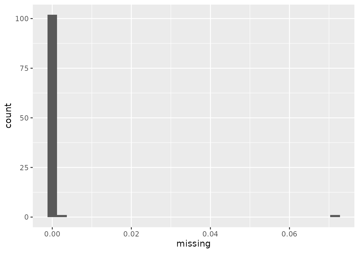
Visualize Genotype Data
We can also plot a histogram of genotypic values using
plot_genotype_histogram().
plot_genotype_histogram(filtered_geno)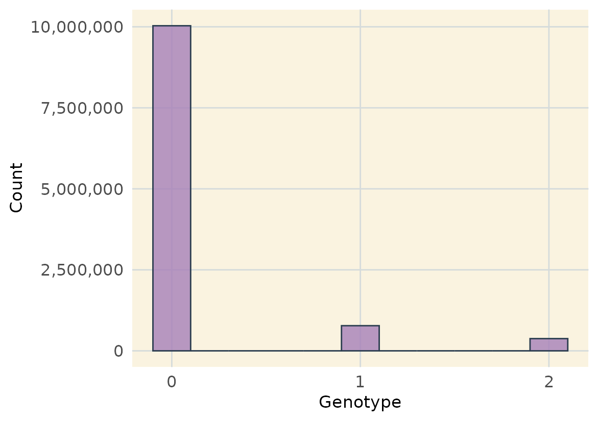
Let’s also take a look at the coverage of the markers across the
genome and chromosomes. This function is based on MapRtool’s
plot_coverage. I just added a few customization. Check it
out here.
Because our filtered genotype matrix has the marker names in the row
names in the format “CHR7_192222” we can use the function
extract_map() from geneticMapR to easily
create a physical map with columns “marker” “chrom” and “position”.
The function extract_map() is very flexible but the row
names should contain components (chromosome, position) separated by a
symbol (e.g., _, -, .). Use arguments chrom_index and
pos_index to specify their positions, and split_symbol to
define the delimiter.
In our example “CHR7_192222”,
chrom_index = 1 as the chromosome is the first field before
the delimiter “_“. If our markers were coded as
W257B_“CHR7_192222” then chrom_index = 2
and pos_index = 3 as chromosome and position are in the
second and third field respectively.
extract_map is tested to work with the symbols “_“,”-”
and “.”. Other valid separators may also be valid
# Extract physical map
map <- extract_map(genotype_matrix = filtered_geno,
                   chrom_index = 1, # Index for Chromosome
                   pos_index = 2,
                    markers = FALSE,  # If TRUE, includes original marker names
                    split_symbol = "_")
Let’s see the first few lines of the map
# See map heading
head(map)
#>   chrom position
#> 1  CHR7   192222
#> 2  CHR7   192239
#> 3  CHR7   192241
#> 4  CHR7   192273
#> 5  CHR7   225702
#> 6  CHR7   225710
Now we are ready for plotting:
geneticMapR::plot_cover(map=map, customize = TRUE)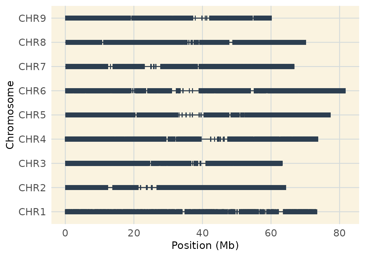
Genotype Frequency
We can evaluate genotype frecuency using the freq()
function. The function computes the relative frequency of each genotype
(typically coded as 0, 1, or 2) across markers or individuals.
Genotype Frequency by Marker
We first calculate genotype frequencies by marker:
geno.freq.mar <- freq(filtered_geno, input_format = "numeric", by = "markers")This returns the relative frequency of each genotype (0, 1, 2) at each marker locus across all individuals, allowing identification of loci with high homozygosity or heterozygosity.
It can also help to filter out markers downstream.
Let’s take a look
head(geno.freq.mar)
#>                 0         1         2
#> CHR7_192222 0.125 0.5288462 0.3461538
#> CHR7_192239 1.000 0.0000000 0.0000000
#> CHR7_192241 1.000 0.0000000 0.0000000
#> CHR7_192273 1.000 0.0000000 0.0000000
#> CHR7_225702 1.000 0.0000000 0.0000000
#> CHR7_225710 1.000 0.0000000 0.0000000
Genotype Frequency by Marker
To evaluate genotype frequncies for individuals across all markers:
geno.freq.ind <- freq(filtered_geno, input_format = "numeric", by = "individuals")This produces the relative frequency of each genotype for every individual, helping to pinpoint individuals with unusually high or low homozygosity levels.
Let’s take a look
head(geno.freq.ind)
#>                          0          1          2
#> 7001-F1-Beta-H9  0.8822163 0.09591408 0.02186960
#> 2001-F2-Beta-A10 0.8940523 0.07536372 0.03058399
#> 2002-F2-Beta-B10 0.9041417 0.05869674 0.03716160
#> 2003-F2-Beta-C10 0.8998198 0.06497826 0.03520198
#> 2004-F2-Beta-D10 0.9027175 0.05645933 0.04082315
#> 2005-F2-Beta-E10 0.8934391 0.07540088 0.03116000
Marker Type Analysis
Markers can be classified based on the genotypes of two parents:
- Homozygous: Fixed for either one allele (P1 = 0 & P2 = 2 or P1 = 2 & P2 = 0:)
- Non-polymorphic: Both parents have the same genotype (e.g., P1 = P2 = 0, 1, or 2)
- Heterozygous: One or both parents are heterozygous (e.g., P1 = 1 & P2 = 0)
Non-polymorphic markers should always be removed. Heterozygous markers can optionally be excluded depending on your analysis goals.
To filter out heterozygous markers and keep only homozygous markers,
we can use filter_geno_by_parents().
# Declare the name of the parents as they appear in the column of your geno
P1 <- "P2550-Cylindra-P1-Theta-A9"
P2 <- "P2493-Mono-P2-Theta-B9"

# Run our function to fiter out heterozygous markers
geno_homozygous <- filter_geno_by_parents(filtered_geno, P1, P2)
P1 and P2 are the column names for the
parental genotypes. filter_geno_by_parents retains only
homozygous polymorphic markers between two specified parents.
Note: The recode_markers()function also
performs this filtering automatically. The user can specify also if
recode_markers()should keep het markers or not. Let’s
see.
Recode Genotypes
geneticMapR::recode_markers() is the heart of the
package. This powerful function phases or recodes genotype marker data
based on two parental references (arguments parent1 and
parent2).
Recoding markers is one of the key steps in genetic mapping. The markers are coded in a way such that the haplotypes coming from either parent can be tracked in the F2 progeny.
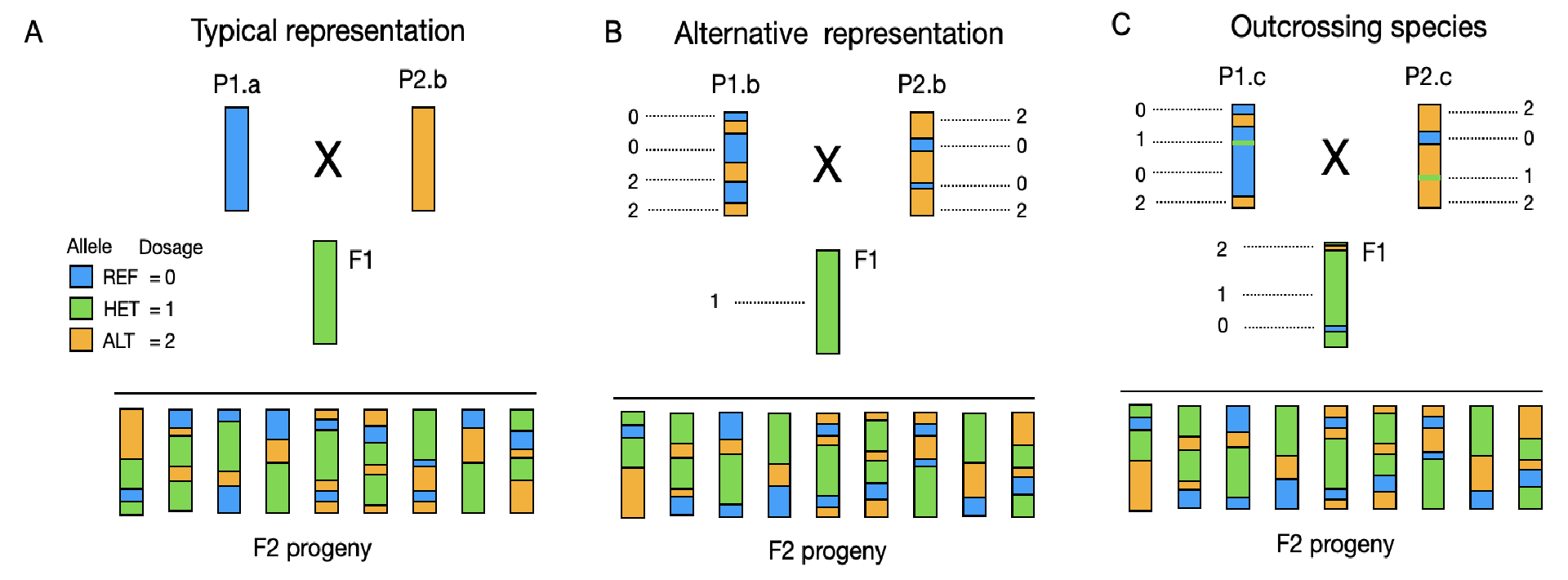
Typical representation
In the figure above panel A is a typical representation of an intercross to derive an F2 mapping population. The parental lines are usually shown as fully homozygous:
- P1.a carries only the reference allele (blue, dosage = 0).
- P2.b carries only the alternate allele (orange, dosage = 2).
The resulting F1 is heterozygous (green, dosage = 1) at all loci.
F2 individuals show a segregating mix of genotypes (0, 1, 2).
This representation is valid when one your parents is the reference genome used to call SNPs. If that is the case then no recoding needs to occur. However, that is a rather rare case.
Alternative representation
In this representation, parental genotypes, are assumed to be homozygous but are fixed for different alleles across loci, allowing for more complex and realistic representations:
- P1.b and P2.b carry both homozygous dosage values (0, or 2). Still homozygous but fixed for different alleles.
Outcrossing species
Most often and in outcrossing species like carrot and table beets or others with high heterozygosity, the (inbred) parents may have mixed genotypes with not totally homozygous genotypes. This is because some loci are lethal on either homozygous configuration.
- P1.c and P2.c carry some heterozygous markers (1) in a low proportion, with homozygous dosage values of 0 or 2.
F1s are mostly heterozygous, but due to genotyping error or residual heterozygosity some dosages of 0 and 2 are typically observed in these individuals
Recode function
recode_markers() was created to help with the task of
recoding the markers so that they reflect a the “typical
representation”. This helps the user track the origin of the haplotypes
in the F2. Essential for genetic mapping.
The function is quite flexible and its main functionality is:
- Drop markers where either of the parent is NA
- Remove non-polymorphic markers automatically (both parents have the same genotype)
- If
handle_het_markers= TRUE, allows parental heterozygous markers to be kept.
Note: there are different types of Het markers. Please see the function documentation for more information.
# Retains only homozygous markers
hom_phased_geno_1629 <- geneticMapR::recode_markers(geno = filtered_geno,
                                parent1 = P1,
                                parent2 = P2,
                                numeric_output = TRUE,
                                handle_het_markers = FALSE)
#> Dropping markers with NA in at least one of the parents. Your genotype matrix contains missing parental genotypes.
#> Dropping non-polymorphic markers. Your genotype matrix contains markers that are identical in the two parents.

# Allows for heterozygous markers
het_phased_geno_1629 <- geneticMapR::recode_markers(geno = filtered_geno,
                               parent1 = P1,
                               parent2 = P2,
                               numeric_output = TRUE,
                               handle_het_markers = TRUE)
#> Dropping markers with NA in at least one of the parents. Your genotype matrix contains missing parental genotypes.
#> Dropping non-polymorphic markers. Your genotype matrix contains markers that are identical in the two parents.
Below is an example of how recode_markers() works. Is
based on simulated data for convenience.
# Load the example dataset
data("simulated_geno")

# Check markers previous to recoding
print(simulated_geno)
#>         Parent1 Parent2 F2_1 F2_2 F2_3
#> Marker1       0       2    0    1    2
#> Marker2       2       0    2    0    1
#> Marker3       0       2    1    2    1
#> Marker4       2       0    2    0    0
#> Marker5       0       2    0    2    1
#> Marker6       2       0    2    0    0

# Recode the markers using the recode_markers() function
phased <- geneticMapR::recode_markers(simulated_geno, parent1 = "Parent1", parent2 = "Parent2")

# Print the output
print(phased)
#>         Parent1 Parent2 F2_1 F2_2 F2_3
#> Marker1       0       2    0    1    2
#> Marker2       0       2    0    2    1
#> Marker3       0       2    1    2    1
#> Marker4       0       2    0    2    2
#> Marker5       0       2    0    2    1
#> Marker6       0       2    0    2    2
Tradeoff Between Marker Type and Genome Coverage
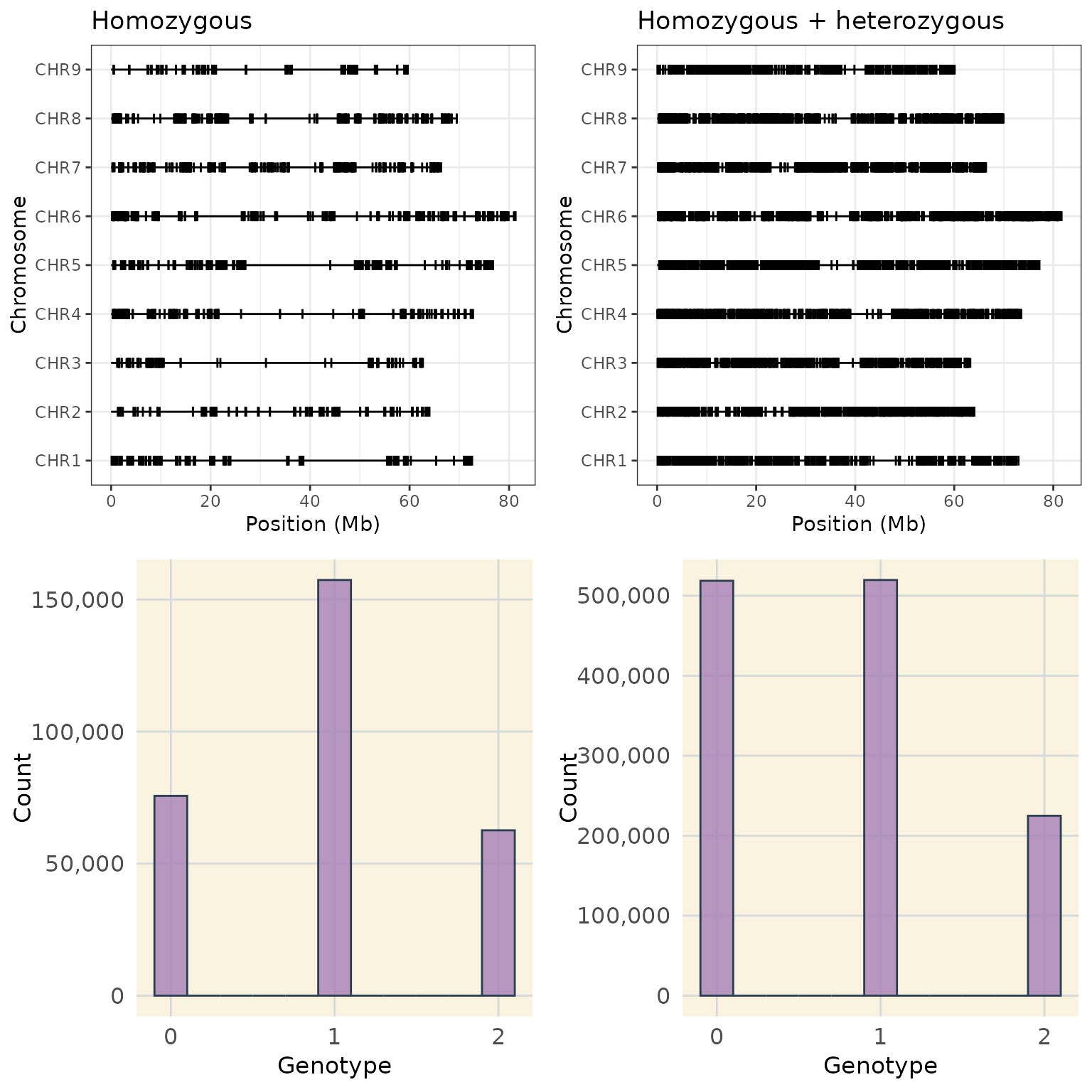
In outcrossing species I have noticed a tradeoff between coverage and the quantity of heterozygous markers.
Including heterozygous markers increases genome coverage compared to using only homozygous markers, but comes with tradeoffs. While heterozygous markers can improve coverage, especially in regions near the centromere, loci with segregation distortion or deleterious alleles, they may complicate downstream linkage group estimation due to their different segregation patterns.
The following section illustrates this tradeoff between marker type and genome coverage.
a <- plot_cover(map = extract_map(hom_phased_geno_1629)) + ggtitle("Homozygous")
b <- plot_cover(map = extract_map(het_phased_geno_1629)) + ggtitle("Homozygous + heterozygous")
c <- plot_genotype_histogram(hom_phased_geno_1629)
d <- plot_genotype_histogram(het_phased_geno_1629)

ggarrange(a, b, c, d,
          nrow = 2,
          ncol = 2
          )
Genotype Frequencies and Filtering
geneticMapR includes functions to estimate frequencies
like freq() in an easy way. The function allows to estimate
genotype frequencies for later filtering.
# Get Frequencies
geno.freq.hom <- freq(hom_phased_geno_1629,  input_format = "numeric", by ="markers")
geno.freq.het <- freq(het_phased_geno_1629, input_format = "numeric", by = "markers")

# Plots
het_plot <- frequency_plot(geno.freq.het) + ggtitle("Het markers, unfiltered")
hom_plot <- frequency_plot(geno.freq.hom) + ggtitle("Hom markers, unfiltered")

# Arrange
ggarrange(hom_plot,
          het_plot,
          nrow = 2)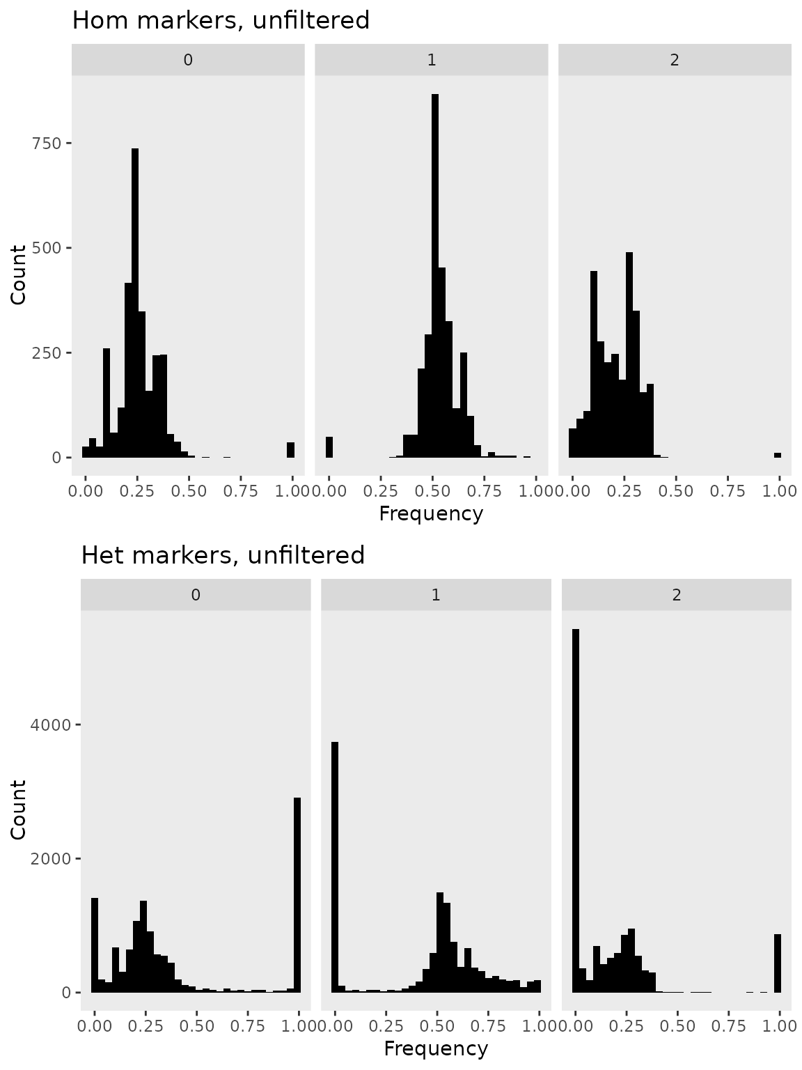
From the plots above we see that there is an abundance of markers at
frequencies of 0 and 1 across all gentoypes (i.e., 0, 1, 2). We can use
the function filter_geno_by_freq() to filter markers out by
maximum genotype frequency and keeping a range of heterozygous
frequencies, say no lower than 0.1 or hiher than 0.70. Which is
reasonable for an F2 mapping populations.
The resulting plot shows a filtered marker set and the overabundance of markers at frequencies of 0 and 1 have been filtered out.
# Heterozygous marker curation
het_phased_geno_1629_filt <- filter_geno_by_freq(het_phased_geno_1629,
                                                 max_geno_freq = 0.90,
                                                 het_freq_range = c(0.1, 0.70)
)

# Create a dataset of frequencies based on the filtered data
geno.freq.het.filtered <- freq(het_phased_geno_1629_filt,
                               input_format = "numeric",
                               by ="markers")


# Create plot
frequency_plot(geno.freq.het.filtered) + ggtitle("Het markers, filtered")
#> `stat_bin()` using `bins = 30`. Pick better value with `binwidth`.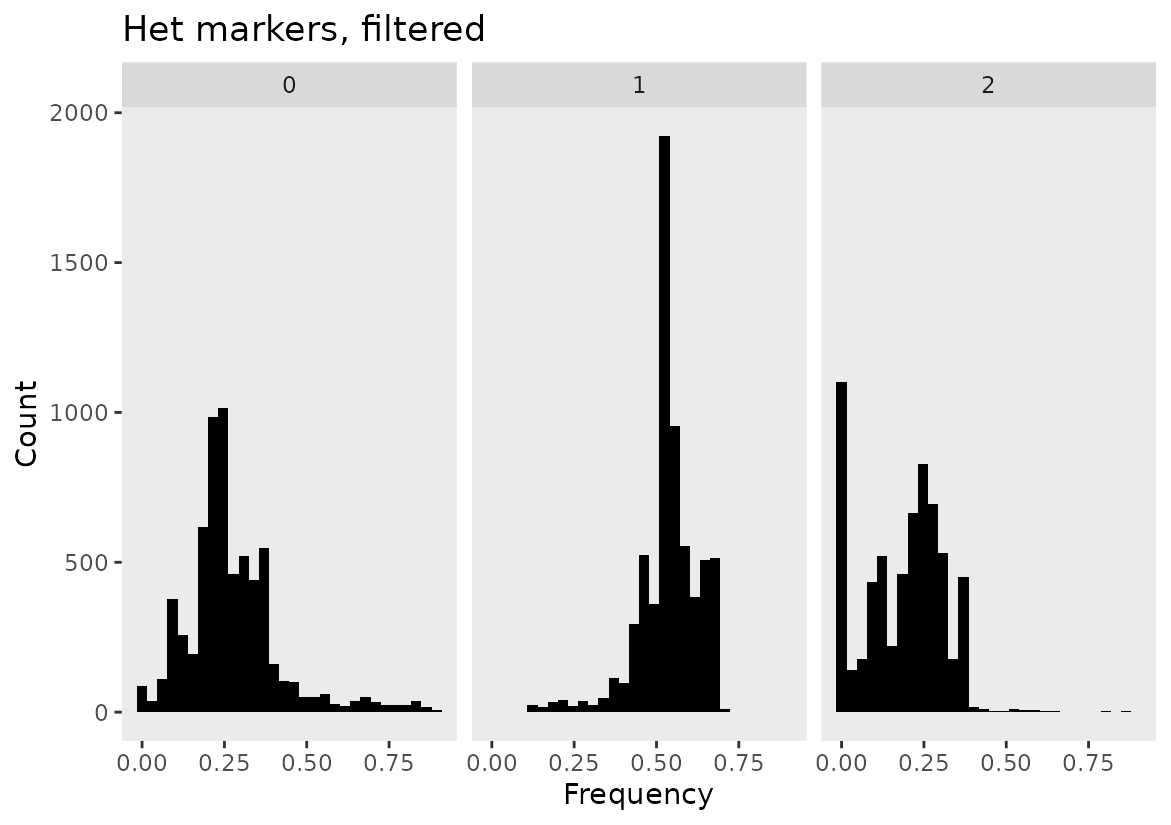
Below we see that our filtering paramaters have left us with a typical 1:2:1 segregation ratio even for markers that included heterozygous markers that were properly filtered.
v <- plot_genotype_histogram(het_phased_geno_1629_filt) +
  ggtitle("Homozygous + filtered het markers")

w <-  plot_genotype_histogram(hom_phased_geno_1629) +
  ggtitle("Homomozygous markers")

ggarrange(v, w,
          nrow = 2)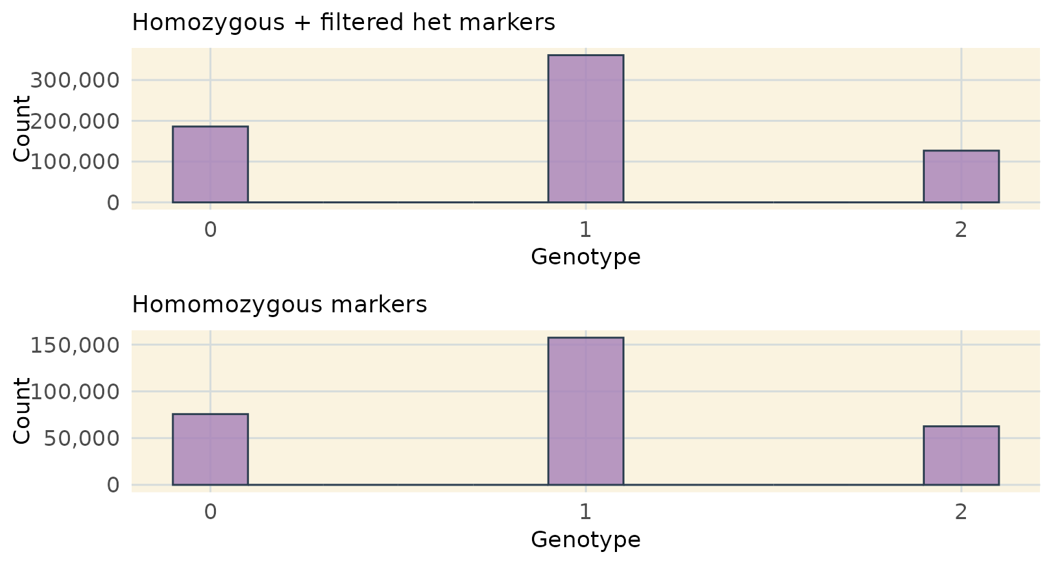
Save Results
save(hom_phased_geno_1629,
     het_phased_geno_1629,
     het_phased_geno_1629_filt,
     file = "processed_data/R_data/filtered_geno_matrices_1629.RData")
Conclusion
A lot of genetic map construction revolves around the type of markers you have and how you make good use of them. Very many filtering steps are taken specially using GBS data to make sure the curated set of markers are markers you can trust and informative.
This vignette provides a workflow for preparing and phasing genotypic
data for genetic mapping analyses in an F2 population using
tools from geneticMapR and other bioinformatics packages.
Let’s continue in the next article the genetic map construction.
Session Information
sessionInfo()
#> R version 4.5.1 (2025-06-13)
#> Platform: x86_64-pc-linux-gnu
#> Running under: Ubuntu 24.04.2 LTS
#>
#> Matrix products: default
#> BLAS:   /usr/lib/x86_64-linux-gnu/openblas-pthread/libblas.so.3
#> LAPACK: /usr/lib/x86_64-linux-gnu/openblas-pthread/libopenblasp-r0.3.26.so;  LAPACK version 3.12.0
#>
#> locale:
#>  [1] LC_CTYPE=C.UTF-8       LC_NUMERIC=C           LC_TIME=C.UTF-8
#>  [4] LC_COLLATE=C.UTF-8     LC_MONETARY=C.UTF-8    LC_MESSAGES=C.UTF-8
#>  [7] LC_PAPER=C.UTF-8       LC_NAME=C              LC_ADDRESS=C
#> [10] LC_TELEPHONE=C         LC_MEASUREMENT=C.UTF-8 LC_IDENTIFICATION=C
#>
#> time zone: UTC
#> tzcode source: system (glibc)
#>
#> attached base packages:
#> [1] grid      stats4    stats     graphics  grDevices utils     datasets
#> [8] methods   base
#>
#> other attached packages:
#>  [1] png_0.1-8                   ggpubr_0.6.1
#>  [3] ggplot2_3.5.2               tibble_3.3.0
#>  [5] tidyr_1.3.1                 dplyr_1.1.4
#>  [7] VariantAnnotation_1.54.1    Rsamtools_2.24.0
#>  [9] Biostrings_2.76.0           XVector_0.48.0
#> [11] SummarizedExperiment_1.38.1 Biobase_2.68.0
#> [13] GenomicRanges_1.60.0        GenomeInfoDb_1.44.0
#> [15] IRanges_2.42.0              S4Vectors_0.46.0
#> [17] MatrixGenerics_1.20.0       matrixStats_1.5.0
#> [19] BiocGenerics_0.54.0         generics_0.1.4
#> [21] MapRtools_0.36              geneticMapR_0.0.0.9000
#>
#> loaded via a namespace (and not attached):
#>  [1] DBI_1.2.3                bitops_1.0-9             rlang_1.1.6
#>  [4] magrittr_2.0.3           RSQLite_2.4.2            compiler_4.5.1
#>  [7] GenomicFeatures_1.60.0   mgcv_1.9-3               systemfonts_1.2.3
#> [10] vctrs_0.6.5              stringr_1.5.1            pkgconfig_2.0.3
#> [13] crayon_1.5.3             fastmap_1.2.0            backports_1.5.0
#> [16] CVXR_1.0-15              labeling_0.4.3           ca_0.71.1
#> [19] rmarkdown_2.29           UCSC.utils_1.4.0         ragg_1.4.0
#> [22] purrr_1.1.0              bit_4.6.0                xfun_0.52
#> [25] cachem_1.1.0             Rmpfr_1.1-1              jsonlite_2.0.0
#> [28] splines2_0.5.4           blob_1.2.4               gmp_0.7-5
#> [31] DelayedArray_0.34.1      BiocParallel_1.42.1      broom_1.0.8
#> [34] parallel_4.5.1           R6_2.6.1                 bslib_0.9.0
#> [37] stringi_1.8.7            RColorBrewer_1.1-3       rtracklayer_1.68.0
#> [40] car_3.1-3                jquerylib_0.1.4          Rcpp_1.1.0
#> [43] iterators_1.0.14         knitr_1.50               Matrix_1.7-3
#> [46] splines_4.5.1            tidyselect_1.2.1         abind_1.4-8
#> [49] yaml_2.3.10              TSP_1.2-5                codetools_0.2-20
#> [52] curl_6.4.0               lattice_0.22-7           withr_3.0.2
#> [55] KEGGREST_1.48.1          evaluate_1.0.4           desc_1.4.3
#> [58] ggdist_3.3.3             pillar_1.11.0            carData_3.0-5
#> [61] foreach_1.5.2            distributional_0.5.0     RCurl_1.98-1.17
#> [64] scales_1.4.0             glue_1.8.0               tools_4.5.1
#> [67] BiocIO_1.18.0            BSgenome_1.76.0          GenomicAlignments_1.44.0
#> [70] ggsignif_0.6.4           registry_0.5-1           XML_3.99-0.18
#> [73] fs_1.6.6                 cowplot_1.2.0            seriation_1.5.7
#> [76] AnnotationDbi_1.70.0     nlme_3.1-168             GenomeInfoDbData_1.2.14
#> [79] restfulr_0.0.16          Formula_1.2-5            cli_3.6.5
#> [82] HMM_1.0.2                textshaping_1.0.1        S4Arrays_1.8.1
#> [85] scam_1.2-19              gtable_0.3.6             rstatix_0.7.2
#> [88] sass_0.4.10              digest_0.6.37            SparseArray_1.8.0
#> [91] rjson_0.2.23             htmlwidgets_1.6.4        farver_2.1.2
#> [94] memoise_2.0.1            htmltools_0.5.8.1        pkgdown_2.1.3
#> [97] lifecycle_1.0.4          httr_1.4.7               bit64_4.6.0-1